Lab
Text Feature Extraction for Classification
Alessandro D. Gagliardi
(adapted from Olivier Grisel's tutorial)
What is scikit-learn?
- Library of Machine Learning algorithms
- Focus on standard methods (e.g. ESL-II, (Elements of Statistical Learning))
- Open Source (BSD)
- Simple
fit / predict / transformAPI - Python / NumPy / SciPy / Cython
- Model Assessment, Selection & Ensembles
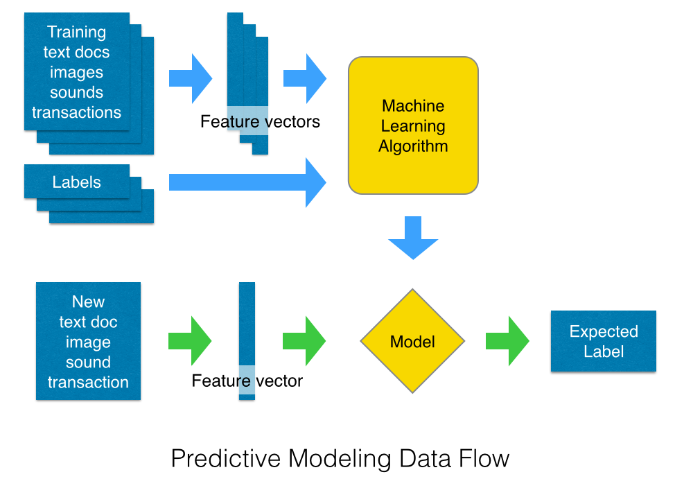
Outline of this section:
- Turn a corpus of text documents into feature vectors using a Bag of Words representation,
- Train a simple text classifier on the feature vectors,
- Wrap the vectorizer and the classifier with a pipeline,
- Cross-validation and model selection on the pipeline.
%matplotlib inline
import matplotlib.pyplot as plt
import numpy as np
import pandas as pd

# Some nice default configuration for plots
plt.rcParams['figure.figsize'] = 10, 7.5
plt.rcParams['axes.grid'] = True
plt.gray()
Check that you have the datasets
%run fetch_data.py
!ls -lh datasets/
Text Classification in 20 lines of Python
Let's start by implementing a canonical text classification example:
- The 20 newsgroups dataset: around 18000 text posts from 20 newsgroups forums
- Bag of Words features extraction with TF-IDF weighting
- Naive Bayes classifier or Linear Support Vector Machine for the classifier itself
from sklearn.datasets import load_files
from sklearn.feature_extraction.text import TfidfVectorizer
from sklearn.naive_bayes import MultinomialNB

# Load the text data
categories = [
    'alt.atheism',
    'talk.religion.misc',
    'comp.graphics',
    'sci.space',
]
twenty_train_small = load_files('datasets/20news-bydate-train/',
    categories=categories, encoding='latin-1')
twenty_test_small = load_files('datasets/20news-bydate-test/',
    categories=categories, encoding='latin-1')

# Turn the text documents into vectors of word frequencies
vectorizer = TfidfVectorizer(min_df=2)
X_train = vectorizer.fit_transform(twenty_train_small.data)
y_train = twenty_train_small.target

# Fit a classifier on the training set
classifier = MultinomialNB().fit(X_train, y_train)
print("Training score: {0:.1f}%".format(
    classifier.score(X_train, y_train) * 100))

# Evaluate the classifier on the testing set
X_test = vectorizer.transform(twenty_test_small.data)
y_test = twenty_test_small.target
print("Testing score: {0:.1f}%".format(
    classifier.score(X_test, y_test) * 100))
Multinomial Naive Bayes
MultinomialNB implements the naive Bayes algorithm for multinomially distributed data, and is one of the two classic naive Bayes variants used in text classification (where the data are typically represented as word vector counts, although tf-idf vectors are also known to work well in practice). The distribution is parametrized by vectors $\theta_y = (\theta_{y1},\ldots,\theta_{yn})$ for each class $y$, where $n$ is the number of features (in text classification, the size of the vocabulary) and $\theta_{yi}$ is the probability $P(x_i \mid y)$ of feature $i$ appearing in a sample belonging to class $y$.
The parameters $\theta_y$ is estimated by a smoothed version of maximum likelihood, i.e. relative frequency counting:
$$ \hat{\theta}_{yi} = \frac{ N_{yi} + \alpha}{N_y + \alpha n} $$
where $N_{yi} = \sum_{x \in T} x_i$ is the number of times feature $i$ appears in a sample of class $y$ in the training set $T$, and $N_{y} = \sum_{i=1}^{|T|} N_{yi}$ is the total count of all features for class $y$.
The smoothing priors $\alpha \ge 0$ accounts for features not present in the learning samples and prevents zero probabilities in further computations. Setting $\alpha = 1$ is called Laplace smoothing, while $\alpha < 1$ is called Lidstone smoothing.
Let's now decompose what we just did to understand and customize each step.
Loading the Dataset
Let's explore the dataset loading utility without passing a list of categories: in this case we load the full 20 newsgroups dataset in memory. The source website for the 20 newsgroups already provides a date-based train / test split that is made available using the subset keyword argument:
ls datasets/
ls -lh datasets/20news-bydate-train
ls -lh datasets/20news-bydate-train/alt.atheism/ | head -n27
The load_files function can load text files from a 2 levels folder structure assuming folder names represent categories:
print(load_files.__doc__)
all_twenty_train = load_files('datasets/20news-bydate-train/',
  encoding='latin-1', random_state=42)
all_twenty_test = load_files('datasets/20news-bydate-test/',
    encoding='latin-1', random_state=42)
all_target_names = all_twenty_train.target_names
all_target_names
all_twenty_train.target
all_twenty_train.target.shape
all_twenty_test.target.shape
len(all_twenty_train.data)
type(all_twenty_train.data[0])
def display_sample(i, dataset):
    print("Class name: " + dataset.target_names[dataset.target[i]])
    print("Text content:\n")
    print(dataset.data[i])
display_sample(0, all_twenty_train)
display_sample(1, all_twenty_train)
Let's compute the (uncompressed, in-memory) size of the training and test sets in MB assuming an 8-bit encoding (in this case, all chars can be encoded using the latin-1 charset).
def text_size(text, charset='iso-8859-1'):
    return len(text.encode(charset)) * 8 * 1e-6

train_size_mb = sum(text_size(text) for text in all_twenty_train.data)
test_size_mb = sum(text_size(text) for text in all_twenty_test.data)

print("Training set size: {0} MB".format(int(train_size_mb)))
print("Testing set size: {0} MB".format(int(test_size_mb)))
If we only consider a small subset of the 4 categories selected from the initial example:
train_small_size_mb = sum(text_size(text) for text in twenty_train_small.data)
test_small_size_mb = sum(text_size(text) for text in twenty_test_small.data)

print("Training set size: {0} MB".format(int(train_small_size_mb)))
print("Testing set size: {0} MB".format(int(test_small_size_mb)))
Extracting Text Features
- Terms that occur in only a few documents are often more valuable than ones that occur in many – inverse document frequency (${IDF}_j$)
- The more often a term occurs in a document, the more likely it is to be important for that document – term frequency (${TF}_{ij}$)
from sklearn.feature_extraction.text import TfidfVectorizer

TfidfVectorizer()
vectorizer = TfidfVectorizer(min_df=1)

%time X_train_small = vectorizer.fit_transform(twenty_train_small.data)
The results is not a numpy.array but instead a scipy.sparse matrix. (Similar to the DocumentTermMatrix in R's tm library.) This datastructure is quite similar to a 2D numpy array but it does not store the zeros.
X_train_small
scipy.sparse matrices also have a shape attribute to access the dimensions:
n_samples, n_features = X_train_small.shape
This dataset has around 2000 samples (the rows of the data matrix):
n_samples
This is the same value as the number of strings in the original list of text documents:
len(twenty_train_small.data)
The columns represent the individual token occurrences:
n_features
This number is the size of the vocabulary of the model extracted during fit in a Python dictionary:
type(vectorizer.vocabulary_)
len(vectorizer.vocabulary_)
The keys of the vocabulary_ attribute are also called feature names and can be accessed as a list of strings.
len(vectorizer.get_feature_names())
Here are the first 10 elements (sorted in lexicographical order):
vectorizer.get_feature_names()[:10]
Let's have a look at the features from the middle:
vectorizer.get_feature_names()[n_features / 2:n_features / 2 + 10]
Training a Classifier on Text Features
We have previously extracted a vector representation of the training corpus and put it into a variable name X_train_small. To train a supervised model, in this case a classifier, we also need
y_train_small = twenty_train_small.target
y_train_small.shape
We can shape that we have the same number of samples for the input data and the labels:
X_train_small.shape[0] == y_train_small.shape[0]
We can now train a classifier, for instance a Multinomial Naive Bayesian classifier:
from sklearn.naive_bayes import MultinomialNB

clf = MultinomialNB(alpha=0.1)
clf
clf.fit(X_train_small, y_train_small)
We can now evaluate the classifier on the testing set. Let's first use the builtin score function, which is the rate of correct classification in the test set:
X_test_small = vectorizer.transform(twenty_test_small.data)
y_test_small = twenty_test_small.target
X_test_small.shape
y_test_small.shape
clf.score(X_test_small, y_test_small)
We can also compute the score on the train set and observe that the model is both overfitting and underfitting a bit at the same time:
clf.score(X_train_small, y_train_small)
Alternative evaluation metrics
Naïve Bayes is a probabilistic models: instead of just predicting a binary outcome (alt.atheism or talk.religion) given the input features it can also estimates the posterior probability of the outcome given the input features using the predict_proba method:
target_predicted_proba = clf.predict_proba(X_test_small)
target_predicted_proba[:5]
By default the decision threshold is 0.5: if we vary the decision threshold from 0 to 1 we could generate a family of binary classifier models that address all the possible trade offs between false positive and false negative prediction errors.
We can summarize the performance of a binary classifier for all the possible thresholds by plotting the ROC curves and quantifying the area under the curve (AUC):
def plot_roc_curve(target_test, target_predicted_proba, categories):
    from sklearn.metrics import roc_curve
    from sklearn.metrics import auc

    for pos_label, category in enumerate(categories):
        fpr, tpr, thresholds = roc_curve(target_test, target_predicted_proba[:, pos_label], pos_label)
        roc_auc = auc(fpr, tpr)
        plt.plot(fpr, tpr, label='{} ROC curve (area = {:.3f})'.format(category, roc_auc))

    plt.plot([0, 1], [0, 1], 'k--')  # random predictions curve
    plt.xlim([0.0, 1.0])
    plt.ylim([0.0, 1.0])
    plt.xlabel('False Positive Rate or (1 - Specifity)')
    plt.ylabel('True Positive Rate or (Sensitivity)')
    plt.title('Receiver Operating Characteristic')
    plt.legend(loc="lower right")
plot_roc_curve(y_test_small, target_predicted_proba, twenty_test_small.target_names)
Here the area under ROC curve ranges between .963 and .974. The ROC-AUC score of a random model is expected to 0.5 on average while the accuracy score of a random model depends on the class imbalance of the data. ROC-AUC can be seen as a way to callibrate the predictive accuracy of a model against class imbalance.
Introspecting the Behavior of the Text Vectorizer
The text vectorizer has many parameters to customize it's behavior, in particular how it extracts tokens:
TfidfVectorizer()
print(TfidfVectorizer.__doc__)
The easiest way to introspect what the vectorizer is actually doing for a given test of parameters is call the vectorizer.build_analyzer() to get an instance of the text analyzer it uses to process the text:
analyzer = TfidfVectorizer().build_analyzer()
analyzer("I love scikit-learn: this is a cool Python lib!")
You can notice that all the tokens are lowercase, that the single letter word "I" was dropped, and that hyphenation is used. Let's change some of that default behavior:
analyzer = TfidfVectorizer(
    preprocessor=lambda text: text,  # disable lowercasing
    token_pattern=ur'(?u)\b[\w-]+\b', # treat hyphen as a letter
                                      # do not exclude single letter tokens
).build_analyzer()

analyzer("I love scikit-learn: this is a cool Python lib!")
The analyzer name comes from the Lucene parlance: it wraps the sequential application of:
- text preprocessing (processing the text documents as a whole, e.g. lowercasing)
- text tokenization (splitting the document into a sequence of tokens)
- token filtering and recombination (e.g. n-grams extraction, see later)
The analyzer system of scikit-learn is much more basic than lucene's though.
Exercise:
- Write a pre-processor callable (e.g. a python function) to remove the headers of the text a newsgroup post.
- Vectorize the data again and measure the impact on performance of removing the header info from the dataset.
- Do you expect the performance of the model to improve or decrease? What is the score of a uniform random classifier on the same dataset?
Hint: the TfidfVectorizer class can accept python functions to customize the preprocessor, tokenizer or analyzer stages of the vectorizer.
type
TfidfVectorizer()alone in a cell to see the default value of the parameterstype
TfidfVectorizer.__doc__to print the constructor parameters doc or?suffix operator on a any Python class or method to read the docstring or even the??operator to read the source code.
Solution:
Let's write a Python function to strip the post headers and only retain the body (text after the first blank line):
def strip_headers(post):
    """Find the first blank line and drop the headers to keep the body"""
    if '\n\n' in post:
        headers, body = post.split('\n\n', 1)
        return body.lower()
    else:
        # Unexpected post inner-structure, be conservative
        # and keep everything
        return post.lower()
Let's try it on the first post. Here is the original post content, including the headers:
original_text = all_twenty_train.data[0]
print(original_text)
Here is the result of applying our header stripping function:
text_body = strip_headers(original_text)
print(text_body)
Let's plug our function in the vectorizer and retrain a naive Bayes classifier (as done initially):
strip_vectorizer = TfidfVectorizer(preprocessor=strip_headers, min_df=2)
X_train_small_stripped = strip_vectorizer.fit_transform(
    twenty_train_small.data)

y_train_small_stripped = twenty_train_small.target

classifier = MultinomialNB().fit(
  X_train_small_stripped, y_train_small_stripped)

print("Training score: {0:.1f}%".format(
    classifier.score(X_train_small_stripped, y_train_small_stripped) * 100))

X_test_small_stripped = strip_vectorizer.transform(twenty_test_small.data)
y_test_small_stripped = twenty_test_small.target
print("Testing score: {0:.1f}%".format(
    classifier.score(X_test_small_stripped, y_test_small_stripped) * 100))
So indeed the header data is making the problem easier (cheating one could say) but naive Bayes classifier can still guess 80% of the time against 1 / 4 == 25% mean score for a random guessing on the small subset with 4 target categories.
Model Selection of the Naive Bayes Classifier Parameter Alone
The MultinomialNB class is a good baseline classifier for text as it's fast and has few parameters to tweak:
MultinomialNB()
print(MultinomialNB.__doc__)
By reading the doc we can see that the alpha parameter is a good candidate to adjust the model for the bias (underfitting) vs variance (overfitting) trade-off.
Setting Up a Pipeline for Cross Validation and Model Selection of the Feature Extraction parameters
The feature extraction class has many options to customize its behavior:
print(TfidfVectorizer.__doc__)
In order to evaluate the impact of the parameters of the feature extraction one can chain a configured feature extraction and classifier:
from sklearn.pipeline import Pipeline

pipeline = Pipeline((
    ('vec', TfidfVectorizer()),
    ('clf', MultinomialNB()),
))
Such a pipeline can then be cross validated or even grid searched:
from sklearn.cross_validation import cross_val_score
from scipy.stats import sem

scores = cross_val_score(pipeline, twenty_train_small.data,
                         twenty_train_small.target, cv=3, n_jobs=3)
scores.mean(), sem(scores)
For the grid search, the parameters names are prefixed with the name of the pipeline step using "__" as a separator:
from sklearn.grid_search import GridSearchCV

parameters = {
    'vec__max_df': [0.8, 1.0],
    'vec__ngram_range': [(1, 1), (1, 2)],
    'clf__alpha': np.logspace(-5, 0, 6)
}

gs = GridSearchCV(pipeline, parameters, verbose=2, refit=False, n_jobs=3)
_ = gs.fit(twenty_train_small.data, twenty_train_small.target)
gs.best_score_
gs.best_params_
Introspecting Model Performance
Displaying the Most Discriminative Features
Let's fit a model on the small dataset and collect info on the fitted components:
pipeline = Pipeline((
    ('vec', TfidfVectorizer(max_df = 0.8, ngram_range = (1, 2), use_idf=True)),
    ('clf', MultinomialNB(alpha = 0.001)),
))
_ = pipeline.fit(twenty_train_small.data, twenty_train_small.target)
vec_name, vec = pipeline.steps[0]
clf_name, clf = pipeline.steps[1]

feature_names = vec.get_feature_names()
target_names = twenty_train_small.target_names

feature_weights = clf.coef_

feature_weights.shape
By sorting the feature weights on the linear model and asking the vectorizer what their names is, one can get a clue on what the model did actually learn on the data:
def display_important_features(feature_names, target_names, weights, n_top=30):
    for i, target_name in enumerate(target_names):
        print(u"Class: " + target_name)
        print(u"")

        sorted_features_indices = weights[i].argsort()[::-1]

        most_important = sorted_features_indices[:n_top]
        print(u", ".join(u"{0}: {1:.4f}".format(feature_names[j], weights[i, j])
                        for j in most_important))
        print(u"...")

        least_important = sorted_features_indices[-n_top:]
        print(u", ".join(u"{0}: {1:.4f}".format(feature_names[j], weights[i, j])
                        for j in least_important))
        print(u"")

display_important_features(feature_names, target_names, feature_weights)
Displaying the per-class Classification Reports
from sklearn.metrics import classification_report

predicted = pipeline.predict(twenty_test_small.data)
print(classification_report(twenty_test_small.target, predicted,
                            target_names=twenty_test_small.target_names))
Printing the Confusion Matrix
The confusion matrix summarize which class where by having a look at off-diagonal entries: here we can see that articles about atheism have been wrongly classified as being about religion 57 times for instance:
from sklearn.metrics import confusion_matrix

pd.DataFrame(confusion_matrix(twenty_test_small.target, predicted),
             index = pd.MultiIndex.from_product([['actual'], twenty_test_small.target_names]),
             columns = pd.MultiIndex.from_product([['predicted'], twenty_test_small.target_names]))
1-2 Pairs
$ unzip Classification_data -d Classification_data
- Load the dateset using
load_files(hint: ourcategoriesare nowspam,easy_ham, etc.) - Write a pre-processor callable to remove the message headers.
- Set up a pipeline for cross validation and model selection using
spamandeasy_ham.- Which parameters should be optimized?
- Do you expect the results to be different from the parameters above? Why/why not?
- Are there other parameters we should optimize that we haven't tested?
- Use
GridSearchCVto find optimal parameters for vectorizor and classifier. - Run classifier against
hard_ham. What percentage ofhard_hamdoes it correctly identify as notspam? - Display the most discriminative features. Anything stick out?
- Run classifier against
spam_2,easy_ham_2,hard_ham_2.- Plot the ROC curve (along with AUC) for each case.
- Print the confusion matrix
Homework
- Read the Naïve Bayes documentation at scikit-learn.org. There are three Naïve Bayes classifiers described. Which of the other two might also be appropriate for this task?
- Explain your choice and apply it to either the spam/ham dataset (if you completed the pair assignment) or the newsgroups dataset (if you didn't).
- Use grid search cross validation to find the best parameters for both the vectorizor and classifier.
- Do different parameters for the vectorizor work better for this classifier?
- Does this classifier do better or worse than the multinomial classifier?
- Advanced: consider the descriptions of the two classifiers in light of which does better for this problem. Can you posit a theory as to why one classifier should do better than the other?