Data Science

Intro to Machine Learning

Alessandro D. Gagliardi

Last Time

What is a regression model?
History of Probability
Descriptive statistics -- numerical
Descriptive statistics -- graphical
p-values and Hypothesis Testing
Inference about a population mean
Difference between two population means

Agenda

What is Machine Learning?
Polynomial and Multiple Linear Regression

Projects

Formal Project Proposals Due Wednesday 5/7

Must include:

README.ml explaining your project in detail
data source and code to access it

What is Machine Learning?¶

from Wikipedia:

Machine learning, a branch of artificial intelligence, is about the construction and study of systems that can learn from data.”

"The core of machine learning deals with representation and generalization..."

representation – extracting structure from data

generalization – making predictions from data

Machine Learning Problems¶

Supervised Learning

Process used for making predictions

Sample data is already classified

Process uses pre-classified information to predict unknown space

Credit: Andrew Ng, "Introduction to Machine Learning," Stanford

Unsupervised Learning

Process used for providing structure

No data was pre "structured", attempts to make sense out of independent variables

(you're making up, or the algorithm is making up, your dependent variable)

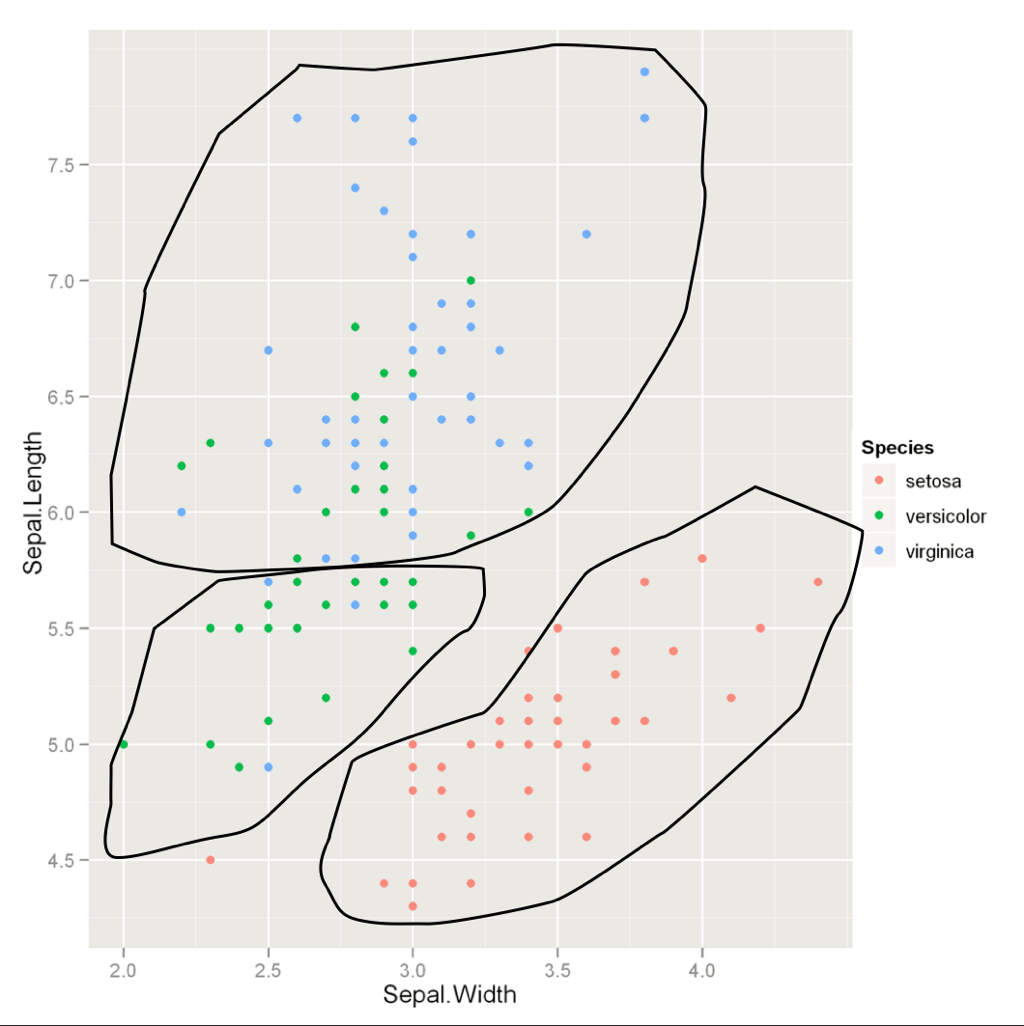
Credit: Thomson Nguyen, "Introduction to Machine Learning," Lookout

The space where data live is called the feature space.

Each point in this space is called a record.

Fitting it all Together¶

What's the goal?

What data do we have?

How do we determine the right approach?

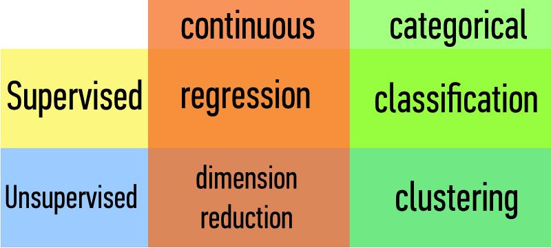
We will implement solutions using models and algorithms.
Each will fall into one of these four buckets.

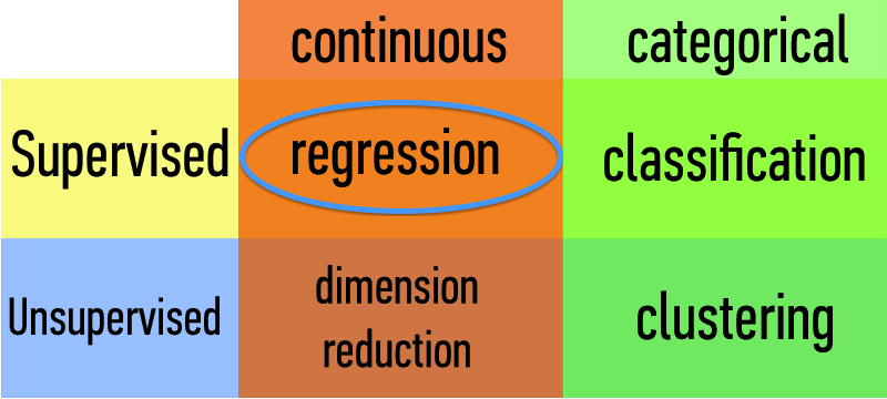
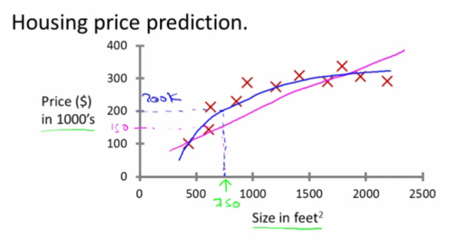
Common linear regression model data problems

I know the prices for all of these other apartments in my area. What could I get for mine?

What's the relationship between total number of friends, posting activity, and the number of likes a new post would get on Facebook?

Careful! Time series data (believe it or not) does not always handle well with simple regression

Recall:

A regression model is a functional relationship between input & response variables.

$$ y = \alpha + \beta x + \epsilon $$

$y =$ response variable (the one we want to predict)

$x =$ input variable (the one we use to train the model)

$\alpha =$ intercept (where the line crosses the y-axis)

$\beta =$ regression coefficient (the model "parameter")

$\epsilon =$ residual (the prediction error)

Ordinary Least Squares

Q. How do we fit a regression model to a dataset?

A. Minimize the sum of the squared residuals (OLS)

$$ min(||y – \beta x||^2) $$

Aside

Why least squares?

We want to penalize both positive and negative residuals.

But why squares and not, say, absolute values?

In fact, in the late 18th century, both of these were considered. OLS won because of procedures making it easier to compute by hand. Today, OLS dominates largely for historical reasons though it is also helpful as it allows a direct comparison between the square of the residuals and the square of the standard deviation (or variance) of the model.

That said, minimizing absolute values may be prefered in cases where there are outliers. (Why?)

Polynomial Regression

Polynomial regression allows us to fit very complex curves to data.
$$ y = \alpha + \beta_1 x + \beta_2 x^2 + \ldots + \beta_n x^n + \epsilon $$

However, it poses one problem, particularly in comparison to simple linear regression

What's the difference between simple linear regression and polynomial regression?

What's the problem that simple regression doesn't have?

Multicollinearity

Multicollinearity is when predictor variables are highly correlated with each other

In [2]:

x = np.arange(1,10.1,0.1)
np.corrcoef(x**9, x**10)[0,1]

Out[2]:

0.99876077218215642

This causes the model to break down because it can't tell the difference between predictor variables

In [3]:

plt.scatter(x**9, x**10)

Out[3]:

<matplotlib.collections.PathCollection at 0x10cc50a90>

How we fix multicollinearity

Replace the correlated predictors with uncorrelated predictors

$$ y = \alpha + \beta_1 f_1(x) + \beta_2 f_2(x^2) + \ldots + \beta_n f_n(x^n) + \epsilon $$

Technical Note: These polynomial functions form an orthogonal basis of the function space.

We will revisit this when we talk about Principal Components Analysis.

Multiple Regression

We can extend this model to several input variables, giving us the multiple linear regression model:

$y = \alpha + \beta_1 x_1 + \ldots + \beta_n x_n + \epsilon$

Prostate data

For more information on the Gleason score.

In [7]:

prostate = com.load_data('prostate')
_ = pd.scatter_matrix(prostate, figsize=(12,6))

Specifying the model

We will use variables lcavol, lweight, age, lbph, svi, lcp and pgg45.
Rather than one predictor, we have $p=7$ predictors.
$$Y_i = \beta_0 + \beta_1 X_{i1} + \dots + \beta_p X_{ip} + \varepsilon_i$$
Errors $\varepsilon$ are assumed independent $N(0,\sigma^2)$, as in simple linear regression.
Coefficients are called (partial) regression coefficients because they “allow” for the effect of other variables.

Fitting the model

Just as in simple linear regression, model is fit by minimizing $$\begin{aligned} SSE(\beta_0, \dots, \beta_p) &= \sum_{i=1}^n(Y_i - (\beta_0 + \sum_{j=1}^p \beta_j \ X_{ij}))^2 \\ &= \|Y - \widehat{Y}(\beta)\|^2 \end{aligned}$$
Minimizers: $\widehat{\beta} = (\widehat{\beta}_0, \dots, \widehat{\beta}_p)$ are the “least squares estimates”: are also normally distributed as in simple linear regression.

In [8]:

mod = smf.ols('lpsa ~ lcavol + lweight + age + lbph + svi + lcp + pgg45', data=prostate)
res = mod.fit()
res.params

Out[8]:

Intercept    0.494155
lcavol       0.569546
lweight      0.614420
age         -0.020913
lbph         0.097353
svi          0.752397
lcp         -0.104959
pgg45        0.005324
dtype: float64

Interpretation of $\beta_j$’s

Take $\beta_1=\beta_{\tt{lcavol}}$ for example. This is the amount the lpsa rating increases for one “unit” of lcavol, keeping everything else constant.
We refer to this as the effect of lcavol allowing for or controlling for the other variables.
For example, let's take the 10th case in our data and change lcavol by 1 unit.

In [11]:

case1 = prostate[9:10]
case2 = case1.copy()
case2.lcavol += 1
yhat = res.predict(pd.concat([case1,case2]))
yhat

Out[11]:

array([ 1.30775437,  1.87730041])

Our regression model says that this difference should be $\hat{\beta}_{\tt lcavol}$.

In [12]:

yhat[1] - yhat[0], res.params['lcavol']

Out[12]:

(0.56954603157399464, 0.56954603157399464)

Goodness of fit for multiple regression

$$\begin{aligned} SSE &= \sum_{i=1}^n(Y_i - \widehat{Y}_i)^2 \\ SSR &= \sum_{i=1}^n(\overline{Y} - \widehat{Y}_i)^2 \\ SST &= \sum_{i=1}^n(Y_i - \overline{Y})^2 \\ R^2 &= \frac{SSR}{SST} \end{aligned}$$

$R^2$ is called the multiple correlation coefficient of the model, or the coefficient of multiple determination.

The sums of squares and $R^2$ are defined analogously to those in simple linear regression.

In [13]:

Y = prostate.lpsa
n = len(Y)
SST = sum((Y - Y.mean())**2)
SSE = sum(res.resid**2)
SSR = SST - SSE
SSR/SST

Out[13]:

0.66300541796546608

Adjusted $R^2$

As we add more and more variables to the model – even random ones, $R^2$ will increase to 1.
Adjusted $R^2$ tries to take this into account by replacing sums of squares by mean squares $$R^2_a = 1 - \frac{SSE/(n-p-1)}{SST/(n-1)} = 1 - \frac{MSE}{MST}.$$

In [14]:

MSE = SSE / res.df_resid
MST = SST / (n - 1)
1 - MSE/MST

Out[14]:

0.6365002261200533

Goodness of fit test

As in simple linear regression, we measure the goodness of fit of the regression model by $$F = \frac{MSR}{MSE} = \frac{\|\overline{Y}\cdot {1} - \widehat{{Y}}\|^2/p}{\\ |Y - \widehat{{Y}}\|^2/(n-p-1)}.$$
Under $H_0:\beta_1 = \dots = \beta_p=0$, $$F \sim F_{p, n-p-1}$$ so reject $H_0$ at level $\alpha$ if $F > F_{p,n-p-1,1-\alpha}.$

In [15]:

MSR = SSR / (n - 1 - res.df_resid)
MSR / MSE

Out[15]:

25.01417163219709

In [16]:

print res.summary()

                            OLS Regression Results                            
==============================================================================
Dep. Variable:                   lpsa   R-squared:                       0.663
Model:                            OLS   Adj. R-squared:                  0.637
Method:                 Least Squares   F-statistic:                     25.01
Date:                Tue, 29 Apr 2014   Prob (F-statistic):           1.54e-18
Time:                        19:55:26   Log-Likelihood:                -98.303
No. Observations:                  97   AIC:                             212.6
Df Residuals:                      89   BIC:                             233.2
Df Model:                           7                                         
==============================================================================
                 coef    std err          t      P>|t|      [95.0% Conf. Int.]
------------------------------------------------------------------------------
Intercept      0.4942      0.874      0.566      0.573        -1.242     2.230
lcavol         0.5695      0.086      6.634      0.000         0.399     0.740
lweight        0.6144      0.198      3.096      0.003         0.220     1.009
age           -0.0209      0.011     -1.905      0.060        -0.043     0.001
lbph           0.0974      0.058      1.691      0.094        -0.017     0.212
svi            0.7524      0.238      3.159      0.002         0.279     1.226
lcp           -0.1050      0.089     -1.175      0.243        -0.282     0.073
pgg45          0.0053      0.003      1.573      0.119        -0.001     0.012
==============================================================================
Omnibus:                        0.550   Durbin-Watson:                   1.543
Prob(Omnibus):                  0.759   Jarque-Bera (JB):                0.175
Skew:                           0.018   Prob(JB):                        0.916
Kurtosis:                       3.205   Cond. No.                         875.
==============================================================================

Inference for multiple regression¶

Regression function at one point

One thing one might want to learn about the regression function in the supervisor example is something about the regression function at some fixed values of ${X}_{1}, \dots, {X}_{6}$, i.e. what can be said about $$ \begin{aligned} \beta_0 + 1.3 \cdot \beta_1 &+ 3.6 \cdot \beta_2 + 64 \cdot \beta_3 + \\ 0.1 \cdot \beta_4 &+ 0.2 \cdot \beta_5 - 0.2 \cdot \beta_6 + 25 \cdot \beta_7 \tag{*}\end{aligned}$$ roughly the regression function at “typical” values of the predictors.

The expression above is equivalent to $$\sum_{j=0}^7 a_j \beta_j, \qquad a=(1,1.3,3.6,64,0.1,0.2,-0.2,25).$$

Confidence interval for $\sum_{j=0}^p a_j \beta_j$

Suppose we want a $(1-\alpha)\cdot 100\%$ CI for $\sum_{j=0}^p a_j\beta_j$.
Just as in simple linear regression:

$$\sum_{j=0}^p a_j \widehat{\beta}_j \pm t_{1-\alpha/2, n-p-1} \cdot SE\left(\sum_{j=0}^p a_j\widehat{\beta}_j\right).$$

statsmodels' will form these coefficients for each coefficient separately when using the conf_int function. These linear combinations are of the form $$ a_{\tt lcavol} = (0,1,0,0,0,0,0,0) $$ so that $$ a_{\tt lcavol}^T\widehat{\beta} = \widehat{\beta}_1 = {\tt coef(prostate.lm)[2]} $$

In [17]:

print res.conf_int(alpha=.1)

                  0         1
Intercept -0.957849  1.946158
lcavol     0.426855  0.712237
lweight    0.284566  0.944274
age       -0.039160 -0.002667
lbph       0.001639  0.193066
svi        0.356505  1.148289
lcp       -0.253468  0.043549
pgg45     -0.000301  0.010950

[8 rows x 2 columns]

$T$-statistics revisited

Of course, these confidence intervals are based on the standard ingredients of a $T$-statistic.

Suppose we want to test $$H_0:\sum_{j=0}^p a_j\beta_j= h.$$ As in simple linear regression, it is based on $$T = \frac{\sum_{j=0}^p a_j \widehat{\beta}_j - h}{SE(\sum_{j=0}^p a_j \widehat{\beta\ }_j)}.$$
If $H_0$ is true, then $T \sim t_{n-p-1}$, so we reject $H_0$ at level $\alpha$ if $$\begin{aligned} |T| &\geq t_{1-\alpha/2,n-p-1}, \qquad \text{ OR} \\ p-\text{value} &= {\tt 2*(1-pt(|T|, n-p-1))} \leq \alpha. \end{aligned}$$

statsmodels produces these in the summary of the linear regression model. Again, each of these linear combinations is a vector $a$ with only one non-zero entry like $a_{\tt lcavol}$ above.

In [18]:

print res.summary()

                            OLS Regression Results                            
==============================================================================
Dep. Variable:                   lpsa   R-squared:                       0.663
Model:                            OLS   Adj. R-squared:                  0.637
Method:                 Least Squares   F-statistic:                     25.01
Date:                Tue, 29 Apr 2014   Prob (F-statistic):           1.54e-18
Time:                        19:55:26   Log-Likelihood:                -98.303
No. Observations:                  97   AIC:                             212.6
Df Residuals:                      89   BIC:                             233.2
Df Model:                           7                                         
==============================================================================
                 coef    std err          t      P>|t|      [95.0% Conf. Int.]
------------------------------------------------------------------------------
Intercept      0.4942      0.874      0.566      0.573        -1.242     2.230
lcavol         0.5695      0.086      6.634      0.000         0.399     0.740
lweight        0.6144      0.198      3.096      0.003         0.220     1.009
age           -0.0209      0.011     -1.905      0.060        -0.043     0.001
lbph           0.0974      0.058      1.691      0.094        -0.017     0.212
svi            0.7524      0.238      3.159      0.002         0.279     1.226
lcp           -0.1050      0.089     -1.175      0.243        -0.282     0.073
pgg45          0.0053      0.003      1.573      0.119        -0.001     0.012
==============================================================================
Omnibus:                        0.550   Durbin-Watson:                   1.543
Prob(Omnibus):                  0.759   Jarque-Bera (JB):                0.175
Skew:                           0.018   Prob(JB):                        0.916
Kurtosis:                       3.205   Cond. No.                         875.
==============================================================================

Questions about many (combinations) of $\beta_j$’s

In multiple regression we can ask more complicated questions than in simple regression.
For instance, we could ask whether lcp and pgg45 explains little of the variability in the data, and might be dropped from the regression model.
These questions can be answered answered by $F$-statistics.
Note: This hypothesis should really be formed before looking at the output of summary.
Later we'll see some examples of the messiness when forming a hypothesis after seeing the summary...

Dropping one or more variables

Suppose we wanted to test the above hypothesis Formally, the null hypothesis is: $$ H_0: \beta_{\tt lcp} (=\beta_6) =\beta_{\tt pgg45} (=\beta_7) =0$$ and the alternative is $$ H_a = \text{one of $ \beta_{\tt lcp},\beta_{\tt pgg45}$ is not 0}. $$
This test is an $F$-test based on two models $$\begin{aligned} Full: Y_i &= \beta_0 + \sum_{j=1}^7 \beta_j X_{ij} \beta_j + \varepsilon_i \\ Reduced: Y_i &= \beta_0 + \sum_{j=1}^5 \beta_j X_{ij} + \varepsilon_i \\ \end{aligned}$$
Note: The reduced model $R$ must be a special case of the full model $F$ to use the $F$-test.

$F$-statistic for $H_0:\beta_{\tt lcp}=\beta_{\tt pgg45}=0$

We compute the $F$ statistic the same to compare any models $$\begin{aligned} F &=\frac{\frac{SSE(R) - SSE(F)}{2}}{\frac{SSE(F)}{n-1-p}} \\ & \sim F_{2, n-p-1} \qquad (\text{if $H_0$ is true}) \end{aligned}$$
Reject $H_0$ at level $\alpha$ if $F > F_{1-\alpha, 2, n-1-p}$.

When comparing two models, one a special case of the other (i.e. one nested in the other), we can test if the smaller model (the special case) is roughly as good as the larger model in describing our outcome. This is typically tested using an F test based on comparing the two models. We can use anova_lm to do this.

In [19]:

reduced_lm = smf.ols("lpsa ~ lcavol + lweight + age + lbph + svi", data=prostate).fit()
print anova_lm(reduced_lm, res)

   df_resid        ssr  df_diff   ss_diff         F    Pr(>F)
0        91  44.436682        0       NaN       NaN       NaN
1        89  43.107558        2  1.329124  1.372057  0.258896

[2 rows x 6 columns]

LAB

In the DAT6 folder, from the command line:

git commit -am ...
git checkout gh-pages
git pull
git checkout personal
git merge gh-pages
ipython notebook

Then open DS_Lab06-ML

Supervised	Making predictions
Unsupervised	Extracting structure

supervised	making predictions	generalization
unsupervised	extracting structure	representation