Data Science
Principal Components Analysis (PCA)
a.k.a. Singular Value Decomposition (SVD) a.k.a. Eigenvalue Decomposition (EVD) a.k.a. Empirical Orthogonal Functions (EOF) a.k.a. Karhunen–Loève transform (KLT) a.k.a. Proper Orthogonal Decomposition (POD) a.k.a. the Hotelling transform a.k.a. factor analysis a.k.a. Eckart–Young theorem a.k.a. Schmidt–Mirsky theorem etc.
Alessandro Gagliardi
Recall
Multicollinearity
%load_ext rmagic
%matplotlib inline
import matplotlib.pyplot as plt
import numpy as np
import pandas as pd
x = np.arange(1,10.1,0.1)
plt.figure(figsize=(9, 9))
plt.scatter(x**9, x**10)

Example
Results of the Olympic Heptathlon Competition, Seoul, 1988.
from D. J. Hand, F. Daly, A. D. Lunn, K. J. McConway and E. Ostrowski (1994). A Handbook of Small Datasets, Chapman and Hall/CRC, London
%R data("heptathlon", package = "HSAUR")
import pandas.rpy.common as com
heptathlon = com.load_data('heptathlon')
heptathlon.describe().T
from A Handbook of Statistical Analyses Using R:
To begin it will help to score all the seven events in the same direction, so that ‘large’ values are ‘good’. We will recode the running events to achieve this.
heptathlon.hurdles = heptathlon.hurdles.max() - heptathlon.hurdles
heptathlon.run200m = heptathlon.run200m.max() - heptathlon.run200m
heptathlon.run800m = heptathlon.run800m.max() - heptathlon.run800m
X_heptathlon = heptathlon.icol(range(7))
y_heptathlon = heptathlon.score
print X_heptathlon.corr().applymap('{:.2f}'.format)
One of these things is not like the other. Do you see it?
Scores in of the events with the exception of javelin are correlated with one another.
javelin is considered a 'technical' event while the others are considered 'power'-based events.
Principal Components Analysis (PCA)
PCA was invented multiple times independently to solve different but related problems.
PCA is equivalent to what is known as the singular value decomposition (SVD) of $\bf{X}$ and the eigenvalue decomposition (EVD), a.k.a. the spectral decomposition of $\bf{X^TX}$ in linear algebra.
FYI: SVD and EVD are slightly different and if your linear algebra skills are up to the task, I encourage you to see how they compare, but for our purposes we may treat them as equivalent.
from Wikipedia:
Depending on the field of application, it is also named the discrete Karhunen–Loève transform (KLT) in signal processing, the Hotelling transform in multivariate quality control, proper orthogonal decomposition (POD) in mechanical engineering . . . factor analysis, Eckart–Young theorem (Harman, 1960), or Schmidt–Mirsky theorem in psychometrics, empirical orthogonal functions (EOF) in meteorological science, empirical eigenfunction decomposition (Sirovich, 1987), empirical component analysis (Lorenz, 1956), quasiharmonic modes (Brooks et al., 1988), spectral decomposition in noise and vibration, and empirical modal analysis in structural dynamics.
Factor Analysis differs from PCA in that Factor Analysis tests an a priori model while PCA makes no assumptions about the underlying structure of the data. Other methods mentioned may also differ in minor ways from what follows but they are all mathemtically related.
Why so many names for the same thing?
Principal Components Analysis (PCA)
PCA reveals a fundamental mathematical relationship between variables.
It has many uses, but the ones we are most interested in are:
- transforming collinear variables into orthogonal factors
- dimensionality reduction
Side note: another, arguably better way to orthogonalize vectors is to use Independent Component Analysis (ICA). The main problem with ICA is that you need to know how many independent components there are to begin with. For that reason, its utility is limited and we will focus on PCA.
Dimensionality Reduction
What is dimensionality reduction?
What are the motivations for dimensionality reduction?
What are different ways to perform dimensionality reduction?
Q: What is dimensionality reduction?
A: A set of techniques for reducing the size (in terms of features, records, and/or bytes) of the dataset under examination.
In general, the idea is to regard the dataset is a matrix and to decompose the matrix into simpler, meaningful pieces.
Dimensionality reduction is frequently performed as a pre-processing step before another learning algorithm is applied.
Q: What are the motivations for dimensionality reduction?
The number of features in our dataset can be difficult to manage, or even misleading (e.g. if the relationships are actually simpler than they appear).
- reduce computational expense
- reduce susceptibility to overfitting
- reduce noise in the dataset
- enhance our intuition
Q: What are different ways to perform dimensionality reduction?
A: There are two approaches: feature selection and feature extraction.
feature selection – selecting a subset of features using an external criterion (filter) or the learning algorithm accuracy itself (wrapper)
feature extraction – mapping the features to a lower dimensional space
Feature selection is important, but typically when people say dimensionality reduction, they are referring to feature extraction.
The goal of feature extraction is to create a new set of coordinates that simplify the representation of the data.
This is what we are doing with PCA.
How does it work?
We want to find a new matrix $P$ from original data $X$ so that the covariance matrix of $PX$ is diagonal (i.e. the resulting vectors are all orthogonal to one another) and entries on diagonal are descending order. In the process:
- Maximize the variance.
- Minimize the projection error.
$$ P_{m\times m}X_{m\times n} = Y_{m\times n} $$
If this works out, $Y_{m\times n}$ is out new data set!
- N.B.: The X here is the tranpose of a typical design matrix..
- See the Shlens paper for more info.
- Its goal is to extract the important information from the data and to express this information as a set of new orthogonal variables called principal components.
- A linear transformation! This is a big assumption.
- Is there another basis, which is a linear combination of the original basis, that best re-expresses our data set?
- This transformation will become the principal components of X.
- What does the transformation boil down to?
- Rotation and scale.. so how does that help us?
- What should our P be doing?
- What do we want our Y do look like?
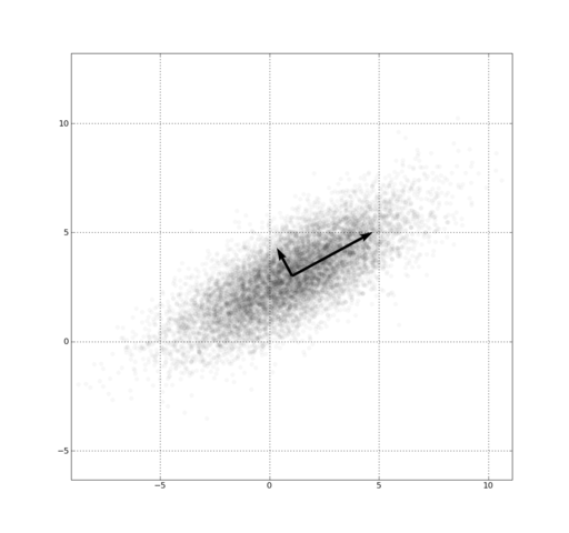
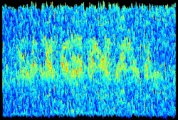
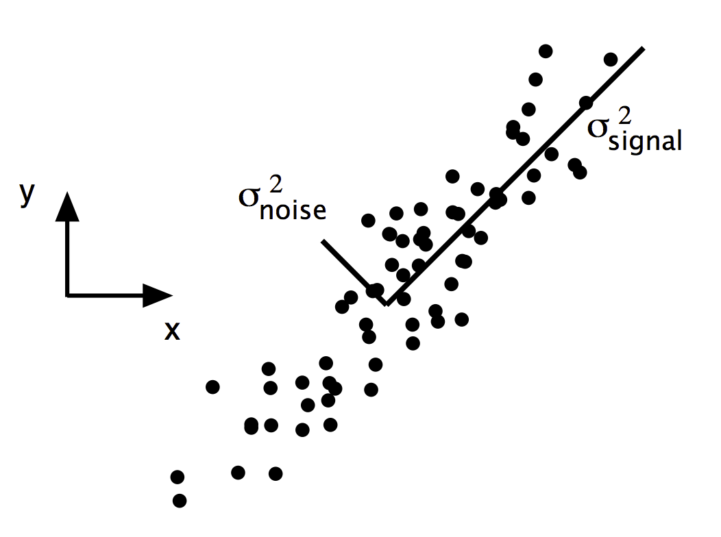
Every dataset has noise and signal... How can we bring out the signal?
$$ SNR = \frac{\sigma^2_{signal}}{\sigma^2_{noise}} $$
Rotate to maximize variance
Heptathlon
_ = pd.scatter_matrix(X_heptathlon, figsize=(8, 8), diagonal='kde')

Principal Components
The hard way:
from __future__ import division

# transpose and scale the original data
scaled_heptathlon = (X_heptathlon - X_heptathlon.mean()) / X_heptathlon.std()
X = np.matrix(scaled_heptathlon.T)

# Calculate P
A = X * X.T
E = np.linalg.eig(A)
P = E[1].T

# Find the new data and standard deviations of the principal components
newdata = P * X
sdev =  np.sqrt((1/(X.shape[1]-1)* P * A * P.T).diagonal())
print "Standard deviations:\n{}".format(sdev)
print "\nRotation:\n{}".format(E[1])
Principal Components
The easy way:
from statsmodels.sandbox.tools.tools_pca import pca
prcomp = pca(X.T)
print "Standard deviations:\n{}".format(np.sqrt(prcomp[2]))
print "\nRotation:\n{}".format(prcomp[3])
def pca_rotations(prcomp, columns=[]):
    if len(columns) <> len(prcomp.components_):
        columns = range(1, len(prcomp.components_) + 1)
    return pd.DataFrame(prcomp.components_,
                        index=(map("PC{}".format, range(1, len(prcomp.components_) + 1))),
                        columns=columns).T
from sklearn.preprocessing import StandardScaler
from sklearn.decomposition import PCA
from sklearn.pipeline import Pipeline

pipeline = Pipeline((
    ('scaler', StandardScaler()),
    ('prcomp', PCA()),
))
pipeline.fit(X_heptathlon.copy())
heptathlon_pca = pipeline.steps[1][1]

print "Standard deviations:\n\t " + ' '.join(map("{:.6}".format, np.sqrt(heptathlon_pca.explained_variance_)))
pca_rotations(heptathlon_pca, X_heptathlon.columns)
_ = pd.scatter_matrix(pd.DataFrame(pipeline.transform(X_heptathlon.copy())), figsize=(8, 8), diagonal='kde')

Notice the scale on each principal component.
Percent Variance Accounted For
def pca_summary(prcomp):
    return pd.DataFrame([np.sqrt(prcomp.explained_variance_),
              prcomp.explained_variance_ratio_,
              prcomp.explained_variance_ratio_.cumsum()],
             index = ["Standard deviation", "Proportion of Variance", "Cumulative Proportion"],
             columns = (map("PC{}".format, range(1, len(prcomp.components_)+1))))
pca_summary(heptathlon_pca)
Visually:
plt.figure(figsize=(10, 7))
plt.bar(range(1, 8), heptathlon_pca.explained_variance_, align='center')

Recall: How we fix multicollinearity with polynomials
Replace the correlated predictors with uncorrelated predictors
$$ y = \alpha + \beta_1 f_1(x) + \beta_2 f_2(x^2) + \ldots + \beta_n f_n(x^n) + \epsilon $$
Technical Note: These polynomial functions form an orthogonal basis of the function space.
Where do Principal Components Come From?
$$ PC_1 = W_{1,1} \times x_1 + W_{1,2} \times x_2 + \cdots + W_{1,n} \times x_n \\ PC_2 = W_{2,1} \times x_1 + W_{2,2} \times x_2 + \cdots + W_{2,n} \times x_n \\ \vdots \\ PC_n = W_{n,1} \times x_1 + W_{n,2} \times x_2 + \cdots + W_{n,n} \times x_n $$
scaled:
$$ PC_1 = W_{1,1} \times \frac{x_1-\bar{x_1}}{\sigma_{x_1}} + W_{1,2} \times \frac{x_2-\bar{x_2}}{\sigma_{x_2}} + \cdots + W_{1,n} \times \frac{x_n-\bar{x_n}}{\sigma_{x_n}} \\ PC_2 = W_{2,1} \times \frac{x_1-\bar{x_1}}{\sigma_{x_1}} + W_{2,2} \times \frac{x_2-\bar{x_2}}{\sigma_{x_2}} + \cdots + W_{2,n} \times \frac{x_n-\bar{x_n}}{\sigma_{x_n}} \\ \vdots \\ PC_n = W_{n,1} \times \frac{x_1-\bar{x_1}}{\sigma_{x_1}} + W_{n,2} \times \frac{x_2-\bar{x_2}}{\sigma_{x_2}} + \cdots + W_{n,n} \times \frac{x_n-\bar{x_n}}{\sigma_{x_n}} $$
Rotations (or Loadings)
These weights are called "rotations" because they rotate the vector space. (They are also called "loadings")
pd.DataFrame(heptathlon_pca.components_, index=(map("PC{}".format, range(1,8))), columns=X_heptathlon.columns).T
Notice:
- the standard devation of each principal component.
- the magnitude of the loadings, particularly the first two components with regard to
javelin.
Annoying side effect: PCA often reverse the sign during decomposition. Keep this in mind because it may reverse your interpretation of the results.
Biplot
Particularly useful for visualizing two principal components compared against each other:
#biplot(heptathlon_pca)
Scaling
- Recall: what is scaling?
- Why is it important? (in other words, why might unscaled variables cause a problem with PCA?)
heptathlon_unscaled_pca = PCA().fit(X_heptathlon.copy())
pca_summary(heptathlon_unscaled_pca)
For comparison:
pca_summary(heptathlon_pca)
At first glance, this looks better than the scaled version. PC1 accounts for 82% of the variance (while in the scaled PCA, PC1 only accounted for 64%).
Similarly, with only two components, we account for 97% of the variance. In the scaled version, the first four components only got us to 95%.
What could go wrong?
X_heptathlon.var()
If one wanted to account for the majority of the overall variance, one need only look at run800m.
In fact, that's exactly what the unscaled PCA does:
pca_rotations(heptathlon_unscaled_pca, X_heptathlon.columns)
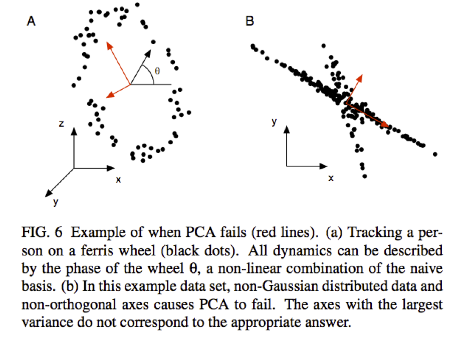
What else could go wrong?
What if the relationship between the variables is nonlinear?
Alternative Uses for PCA
As illustrated by the many names and variations on PCA, this method of analysis has many uses.
e.g. Hanson, S. J., Gagliardi A.D., Hanson, C. (2009). Solving the brain synchrony eigenvalue problem: conservation of temporal dynamics (fMRI) over subjects doing the same task Journal of Cognitive Neuroscience
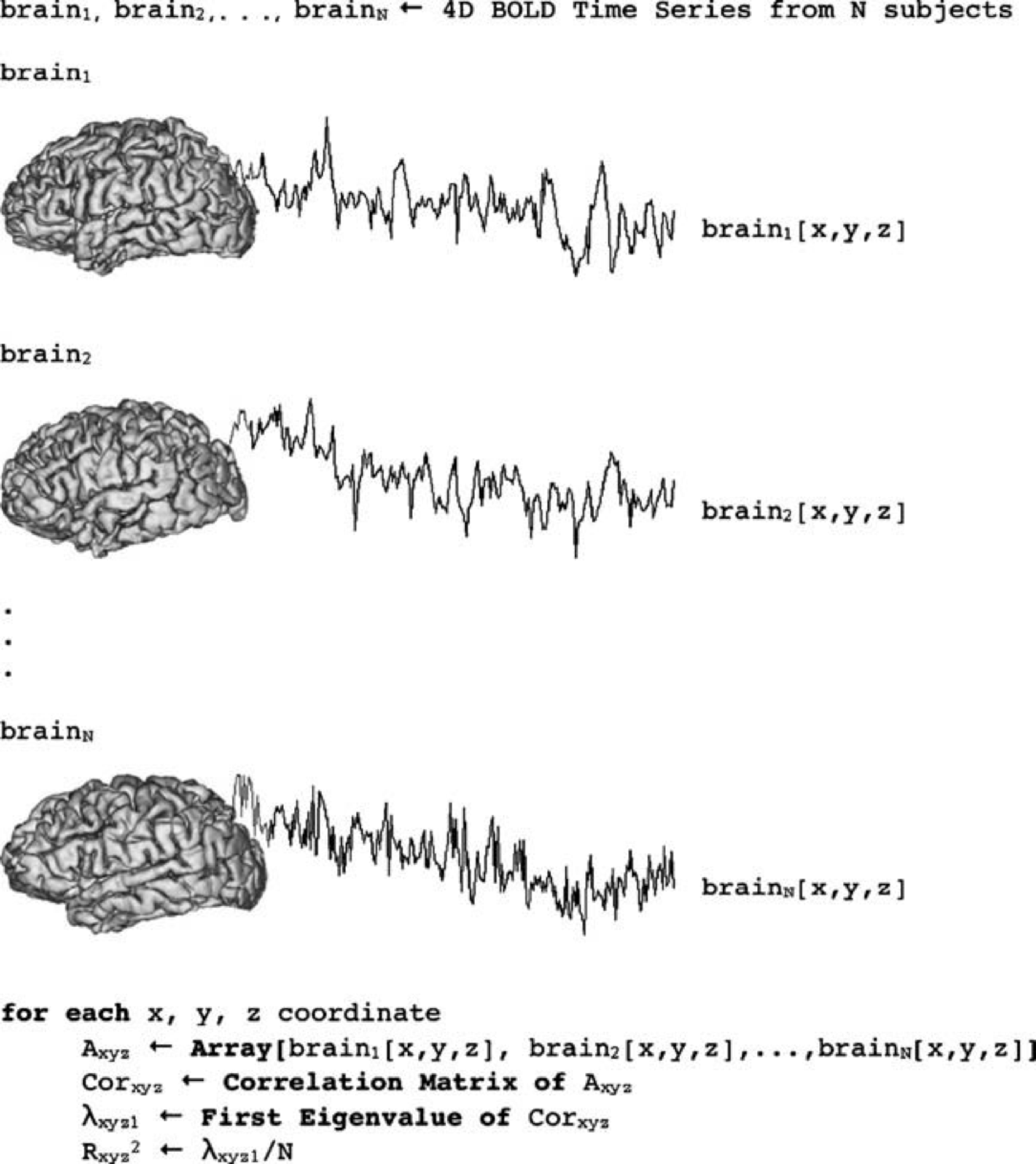
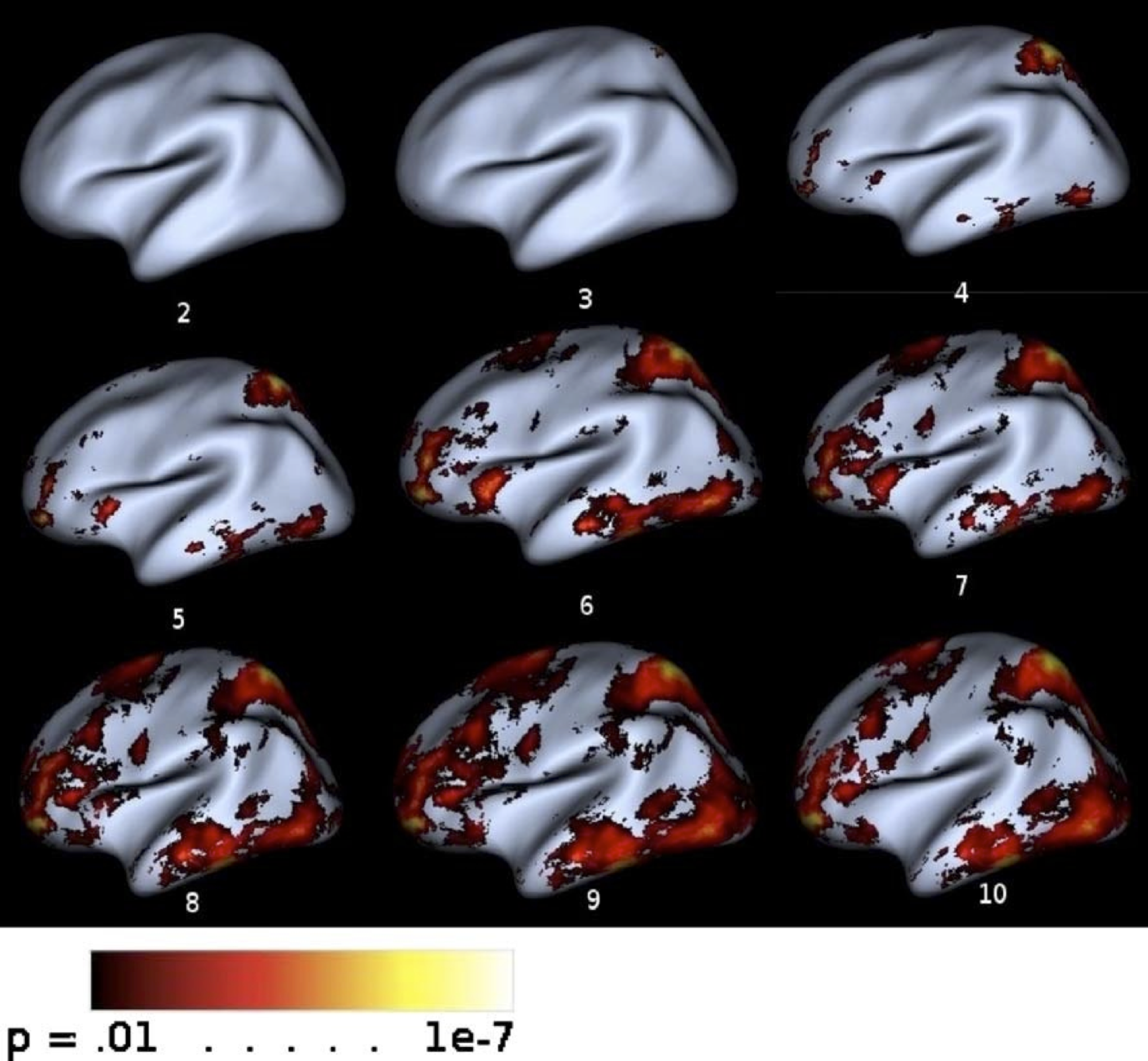
Using Roy’s Largest Root Statistic to determine significance of the percent variance accounted for by the first principal component.
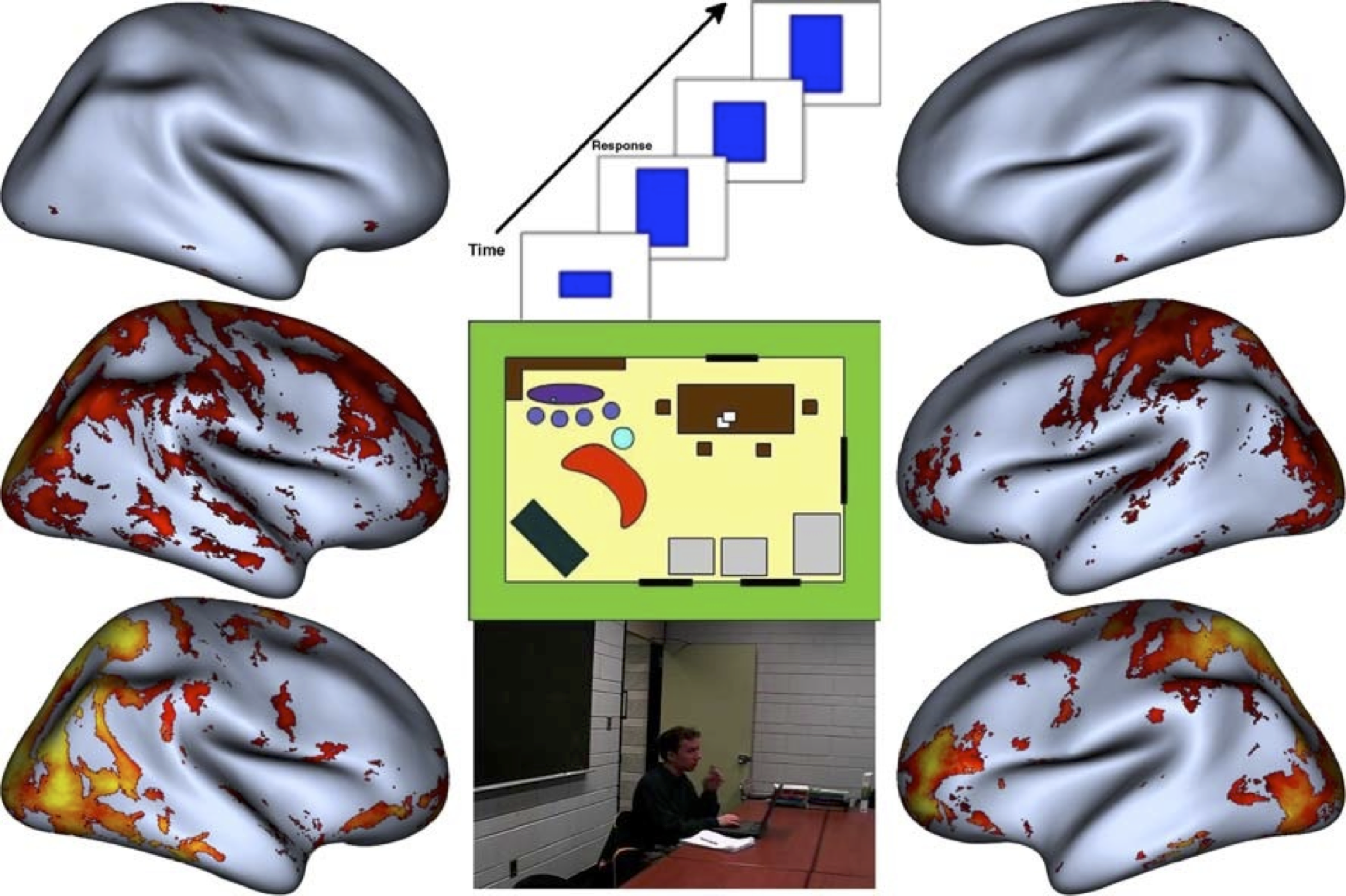
PC1 results as a function of complexity and goal directed aspects of the action sequence.
LAB
In the DAT6 folder, from the command line:
git commit -am ...
git checkout gh-pages
git pull
git checkout personal
git merge gh-pages
ipython notebook
Then open DS_Lab11-PCA